
Data Preparation Workflow Documentation#
Use this guide to run the pre-analysis notebooks in the right order and generate EPM-ready inputs. The primary workflows now live inside pre-analysis/prepare-data/, while pre-analysis/open-data/ remains available whenever you need to refresh the underlying renewable or hydro datasets.
Summary Table#
Step |
Notebook(s) |
Key inputs |
Outputs / Notes |
|---|---|---|---|
1 |
|
Country/zone perimeter |
Defines the modeling scope consumed by every notebook. |
2 |
|
|
Season definitions, precipitation/temperature plots, CSV summaries. |
3 |
|
SPLAT names or coordinates, API keys |
Fresh wind/solar capacity factors when you need to refresh raw inputs before re-running prepare-data notebooks. |
4 |
|
Historical load measurements, monthly means |
Cleaned load history plus synthetic/forecast hourly load profiles. |
4b |
|
Outputs from step 4 |
Shareable demand plots for QA/stakeholder review. |
5 |
|
Climate outputs (step 2), load profiles (step 4), renewables |
|
6 |
|
Hydropower profiles/Atlas tables, |
|
7 |
|
Demand, renewables, hydro availability, generation fleet |
Balance dashboards ensuring supply meets demand before launching GAMS runs. |
Tip: open-data notebooks such as
hydro_inflow.ipynb,hydro_basins.ipynb, andget_generation_maps.ipynbare your toolkit for refreshing the raw datasets that feed the prepare-data workflows above.
1. Define Perimeter Countries/Zones#
Populate
zcmap.csvin the repo root with the countries or zones that match your study.Use consistent SPLAT/EPM names because these IDs drive joins in both
prepare-dataandopen-data.
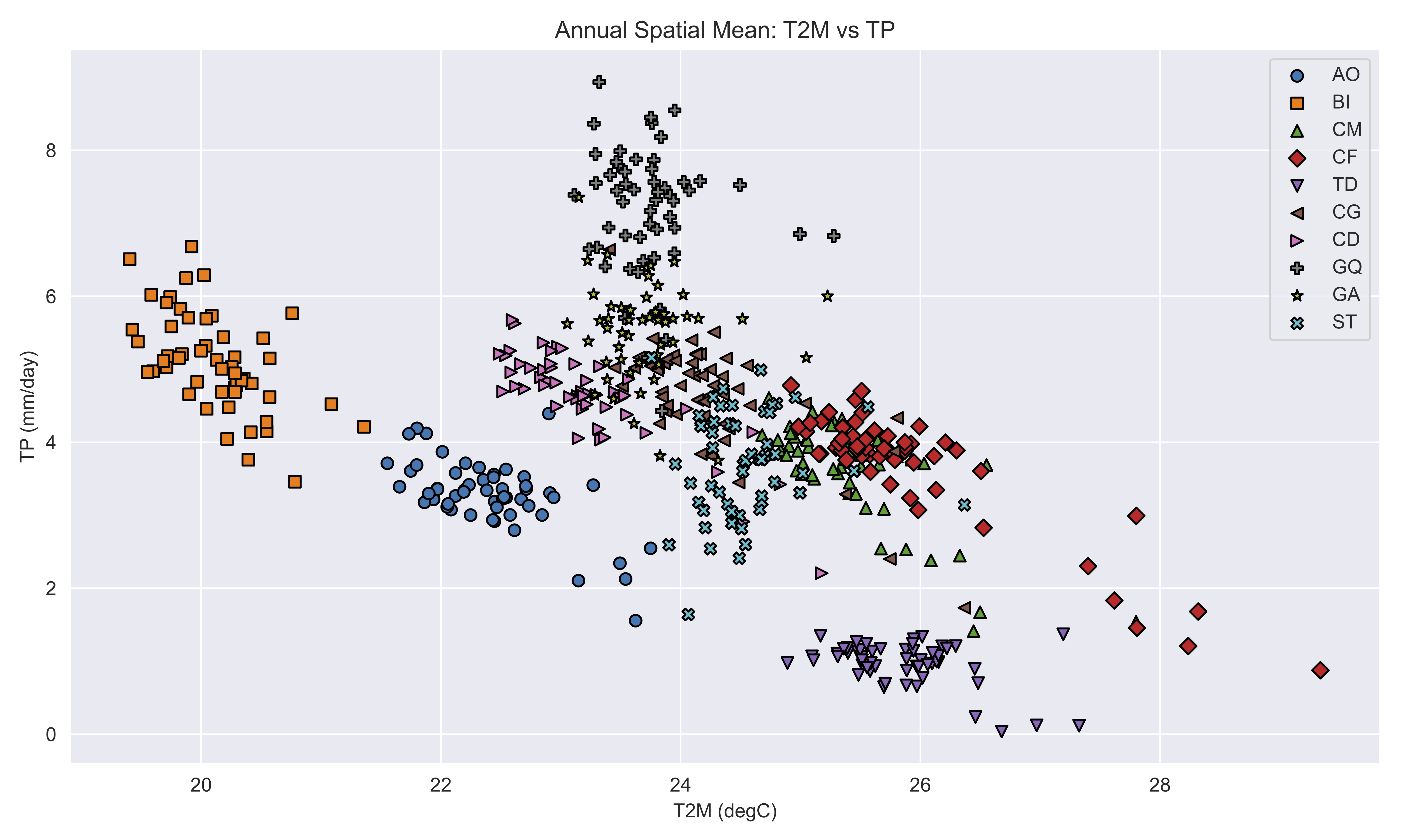
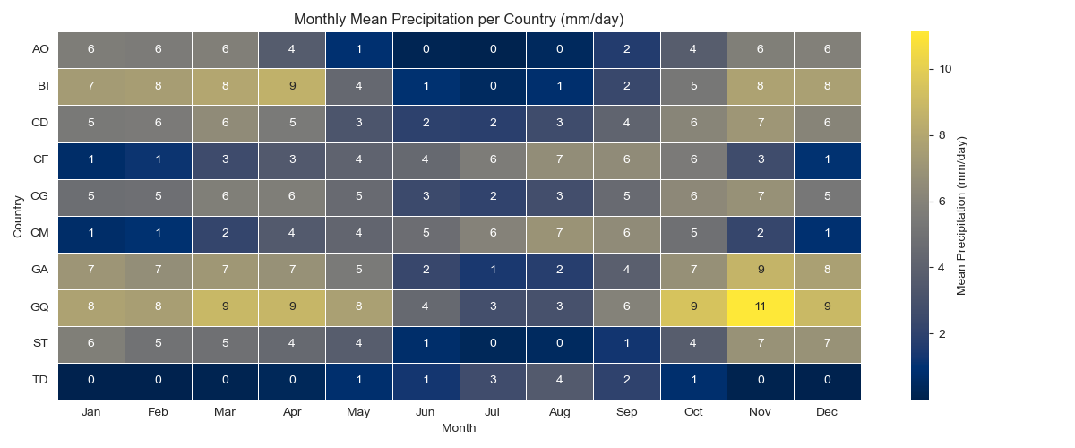
2. Run the Climatic Overview (pre-analysis/prepare-data/climatic_overview.ipynb)#
Objective: quantify precipitation and temperature regimes so you can justify representative seasons or years.
Inputs: zone list from
zcmap.csv, ERA5-Land downloads placed inpre-analysis/prepare-data/input/.Outputs: plots (available under
pre-analysis/prepare-data/output/) and summary CSVs that downstream notebooks read.
3. Refresh Renewable Resource Data (open-data stage)#
When base-year renewable profiles are outdated, switch to pre-analysis/open-data/:
IRENA route —
get_renewables_irena_data.ipynbInputs: list of SPLAT zones plus the IRENA workbook.
Output format:
zone, season, day, hour, <climatic_year>hourly capacity factors.
Renewable Ninja route —
get_renewable_ninja_data.ipynbRequires coordinates from
get_renewables_coordinate.ipynb.Useful for scenario-specific solar/wind traces.
Save the resulting CSVs under pre-analysis/prepare-data/input/ before moving on. You can also use get_generation_maps.ipynb for quick QA plots of the generation fleet.
4. Build Demand Profiles (load_profile_treatment.ipynb, load_profile.ipynb, load_plot.ipynb)#
Treat historical data — run
load_profile_treatment.ipynbto clean utility load logs (remove spikes, fill gaps).Generate the hourly profile — run
load_profile.ipynbto blend treated history with monthly targets or growth assumptions.Plot for QA — use
load_plot.ipynbto export PNG/HTML charts for stakeholder review.
Deliverables: smoothed historical load, modeled hourly demand, and plots placed in pre-analysis/prepare-data/output/.
5. Generate Representative Days (pre-analysis/prepare-data/representative_days/representative_days.ipynb)#
Inputs: load profiles from step 4, renewable capacity-factor tables (step 3), climate summaries (step 2).
Process: cluster the full-year time series into a manageable subset of days while preserving seasonal statistics.
Outputs ready for EPM:
epm/input/data_capp/pHours.csvepm/input/data_capp/load/pDemandProfile.csvepm/input/data_capp/supply/pVREProfile.csv
6. Hydropower Preparation (hydro_availability.ipynb + helpers)#
hydro_availability.ipynbingests monthly hydro profiles or Atlas curves and exports:pAvailabilityCustom.csvfor reservoirs.Run-of-river
pVREgenProfile.csv.
hydro_representative_years.ipynb(optional) samples wet/baseline/dry years before feeding them intohydro_availability.ipynb.Need new inflow data or basin checks? Use the open-data notebooks (
hydro_inflow.ipynb,hydro_basins.ipynb,hydro_atlas_comparison.ipynb) to regenerate the raw profiles, then drop the outputs back intoprepare-data/input/.
7. Supply vs Demand Balance (pre-analysis/prepare-data/supply_demand_balance.ipynb)#
Objective: confirm that the cleaned generation fleet, renewable additions, and hydro schedules cover the demand from step 4.
Inputs:
pGenDataInput_clean.csv, demand/renewable outputs, hydro availability,pHours.Outputs: deficit tables, stacked supply-demand plots, and sanity checks prior to running
epm/main.gms.
Notes#
Keep naming conventions consistent across demand, renewable, and hydro files (zone, technology, scenario).
Store raw downloads in
pre-analysis/open-data/input/orpre-analysis/prepare-data/input/and only copy vetted CSVs intoepm/input.Whenever you introduce a new data vintage, rerun the balance notebook (step 7) before executing the GAMS model.